


Basic Lens Selection
This is Section 6.2 of the Imaging Resource Guide.
How to Choose a Variable Magnification Lens
Types of Machine Vision Lenses explained some of the more common types of imaging lenses to choose from based on the application. In order to narrow down to a more exact choice for an imaging lens, the fundamental system parameters of the imaging system must be known (see Section 1: Lens and Imaging Fundamentals). At a minimum, the working distance (WD), field of view (FOV), and resolution are required constraints before the proper selection of a lens can occur. In this section, it is assumed that a camera has already been chosen, as it narrows down the selection criteria and makes the lens selection easier.
For this discussion, fixed focal length lenses and zoom lenses can be assumed to operate on the same principles and can be chosen in the same fashion. This assumes that zoom lenses are being specified at individual focal lengths and that their zoom functionality has been locked down.
All variable magnification lenses come to a point of focus based upon Equation 1.
Where z' is the image distance (which can be thought of as the distance between the image plane and the last element), z is the object distance (or the distance between the object being focused on and the front lens element), and f is the focal length of the lens. In this version of this equation, the values of z', z, and f should all be positive. Equation 2 is an approximate equation that assumes that the lens has no thickness; it is included here to show the relationship between image and object distances. For a given focal length, as the object distance (WD) increases, the image distance will decrease.
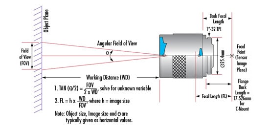
For a single lens element, such as a plano-convex or bi-convex lens, this equation is useful in determining which focal length is proper, given an object and image distance. However, in a machine vision system that uses objectives with many elements (such as those in Figure 1 of Types of Machine Vision Lenses), the equation falls short in several ways: it does not describe the FOV, and since measuring the image distance in a machine vision lens is impractical, solving for focal length becomes impossible.
Using the equation for magnification, Equation 2.
Where H' and H are the size of the image plane (most often a sensor size) and FOV respectively, Equation 1 can be rearranged into a more useful form, shown in Equation 3.
Equation 3 provides a quick and easy way to solve for which focal length lens is required to solve an application, given fundamental parameters such as FOV and sensor size. Often, Equation 3 is shown with the “-1” term dropped, as it is small compared to the rest of the quantity.
The key assumption made in the application of Equation 3 to aid in lens selection is that the camera has already been chosen, and the only variable being solved for is the focal length (f) of the appropriate lens. If this is the case, then lens selection becomes much easier. For example, assume that an FOV of 175mm needs to be achieved with a 500mm WD on an IMX250 sensor (2/3”, 5 MP). Using Equation 3, a 25mm lens is the best choice.
In general, when lens calculators are used online, they are using some form of Equation 3 to generate their answer. Note that these are all first order calculations and will deviate from ideal when lenses with large distortion values are used (such as fisheye lenses), and generally assume that lenses have zero thickness.
Figures 1 and 2 show Equation 3 plotted for several lenses with different focal lengths on different sensors (corresponding to separate y-axes).

Figure 1: Lenses of different focal lengths and their FOVs on ⅓ ” and 1∕1.8” sensors

Figure 2: Lenses of different focal lengths and their FOVs on ⅔ ”and 1” sensors.
These plots are useful in visually determining the proper focal length for a machine vision lens if a camera has already been chosen: simply follow along the x-axis to the required WD and using the corresponding y-axis (depending on the sensor that is being used), find where the points meet on the coordinate plane. The closest lens to the intersecting points describes the best starting point of investigation for which lens to use and considerably narrows the large field of lenses from which to choose.
Additionally, these plots also illustrate several important points about fixed focal length lenses in machine vision. First, longer focal length lenses have longer minimum WDs, which is a consequence of their optical designs. Minimum WD can be shortened by adding spacers between the lens and camera, but image quality will eventually suffer (see Lens Spacers, Shims and Focal Length Extenders). Second, larger sensors provide a larger FOV with the same focal length lens. For example, at a WD of 350mm, a 12mm lens on a ⅔ ” sensor will have a FOV of about 256mm, but on a 1” sensor at the same WD, the FOV is approximately 530mm—an increase of 107%. Lastly, there are gaps in the plots, indicative that a standard off-the-shelf fixed focal length lens does not exist. For example, it is impossible to achieve a 525mm FOV at a 600mm WD with a ⅔” sensor with available focal lengths. The closest lens that exists is an 8.5mm focal length, which would need to be used at a WD of about 510mm to achieve that FOV.
These plots should only be used as the first step in narrowing down which lens is the best for an application. They do not answer questions about image quality, distortion, relative illumination, or any other important qualities of an imaging lens; they merely address FOV relative to sensor size.
How to Choose a Fixed Magnification Lens
At first glance, lenses such as telecentrics or microscope objectives can seem intimidating to specify into an imaging system as they do not behave the same way as traditional fixed focal length lenses. However, the selection process is actually much more straightforward than a traditional lens.
With a few exceptions, fixed magnification lenses generally only function properly at a single WD. They are also specified by their magnification, such as a 2.0X telecentric lens. Because the magnifications are physically listed on the lenses, that is where they always work, and their FOV can by described simply by rearranging Equation 1 from Imaging Fundamentals to:
Where m is the magnification specified for the lens and H is the sensor size. This equation shows that regardless of the sensor size, the magnification will remain the same; only the FOV changes.
For example, an application requires the visual measurement of a bore into a machined part. The bore is 20mm in diameter and the part can vary slightly in placement underneath the imaging system, so a FOV of 24mm is required. A camera has been chosen that has a 1∕1.8” sensor (7.2mm horizontal sensor size), so using Equation 4, the magnification should be 0.3X. Since this is a measurement application, a telecentric lens should be chosen with that magnification.
Note that in the above example, a camera had already been chosen; were a camera not chosen, the lens selection would be more complicated. Advanced Lens Selection spends time discussing how to select a lens when no camera has been chosen.


or view regional numbers
QUOTE TOOL
enter stock numbers to begin
Copyright 2023 | Edmund Optics, Ltd Unit 1, Opus Avenue, Nether Poppleton, York, YO26 6BL, UK
California Consumer Privacy Acts (CCPA): Do Not Sell or Share My Personal Information
California Transparency in Supply Chains Act
This content may include material that has been generated or modified using artificial intelligence (AI).
The FUTURE Depends On Optics®