


MTF Curves and Lens Performance
This is Section 2.6 of the Imaging Resource Guide.
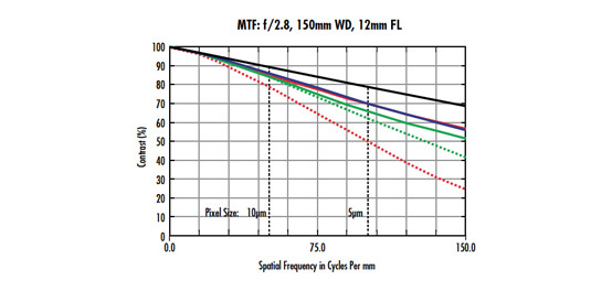
Figure 1 is an example of a modulation transfter function (MTF) curve for a 12mm lens used on the Sony IMX250 sensor (2/3”) format and 3.45µm pixels). Sensor format is described in Sensors. The curve shows lens contrast over a frequency range from 0 to 150$ \small{\tfrac{\text{lp}}{\text{mm}}} $ (the sensor’s limiting/Nyquist resolution is 145$ \small{\tfrac{\text{lp}}{\text{mm}}} ) $. Additionally, this lens has its f/# set at 2.8 and is set at a magnification of 0.05X. The field of view (FOV), approximately 170mm, is about 20X the horizontal dimensions of the sensor. This $ \small{\tfrac{\text{FOV}}{\text{magnification}}} $ will be used for all examples in this section. White light is used for the simulated light source.
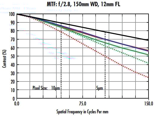
Figure 1: MTF curve for a 12mm lens used in the Sony IMX250 sensor.
This curve provides a variety of information. The first thing to note is that the black diffraction-limited line indicates that the maximum theoretical contrast achievable is almost 70% at the 150 frequency and that no modification to this lens design can make the lens perform better (assuming constant f/# and wavelength). Also important are the blue, green, and red lines which correspond to how this lens performs across the sensor (see The Modulation Transfer Function to see which field positions corresponding to each color). It is shown clearly that, at lower and higher frequencies, contrast reproduction is not the same across the entire sensor, thus, not the same over the FOV.
Comparing Lens Designs and Configurations
Ex. 1: Comparing two lens designs with the same focal length and f/#
Figure 2 examines two different lenses of the same focal length, 12mm, and f/#, f/2.8, on the same sensor, and with the same FOV. These lenses produce systems that are the same size but differ in performance. In analysis, the horizontal light blue line at 30% contrast in Figure 2a shows that at least 30% contrast is achievable nearly across the full FOV, which means full advantage of the sensor is used. For Figure 2b, the full field is nearly below 30% contrast. Better image quality will only be achievable over a small portion of the sensor. Note that the orange box on both curves represents the intercept frequency (at 70% contrast) of the lower performance lens in Figure 2b. When that same box is placed in Figure 2a, a tremendous performance difference between the two lenses can be seen, even at lower frequencies. The reason for the difference between these lenses is the cost associated with both designs and fabrication variations; Figure 2a is associated with a more complex design and tighter manufacturing tolerances. The lens in Figure 2a excels in both lower resolution and higher resolution applications where relatively short working distances (WDs) for larger FOVs are required. Figure 2b will work best where more pixels are needed to enhance the fidelity of image processing algorithms and where lower cost is required. Both lenses are valid designs for situations where they are the correct choice; it depends on the application. Just because a lens does not achieve Nyquist limited resolution on a sensor does not preclude its use on that sensor.


Figure 2: MTF curves for two different lens designs (a and b) with the same focal length, f/#, upon the same sensor, and using the same system parameters.
Ex. 2: Comparing two high-resolution lens designs at the same f/# but different focal lengths
Figure 3 examines two different high-resolution lenses with focal lengths of 12mm and 16mm, and the same FOV, sensor, and f/#. By looking at the lens’s contrast at the Nyquist limit in Figure 3b (the light blue line), a distinct performance increase can be seen compared to Figure 3a. While the absolute difference is only about 25% contrast, the relative difference is closer to 85% considering the change from approximately 25% contrast to 46%. This orange box is placed where Figure 3a hits 70% contrast. Note that the difference in performance in this example is not as extreme as in the previous. The tradeoff between these lenses is that the WD for the lens in Figure 3b has an increase of about 33% but with a decent increase in performance. This follows the general guidelines outlined in Best Practices for Better Imaging.
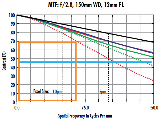
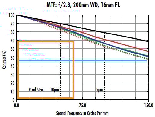
Figure 3: Two different high-resolution lens designs with different focal lengths at the same f/# and system parameters.
Ex. 3: Comparing different f/#s of the same 35mm lens design
Figure 4 features the MTF for a 35mm lens design using white light at f/4 (a) and f/2 (b). The yellow line on both graphs shows the diffraction-limited contrast at the Nyquist limit for Figure 4a while the blue line denotes the lowest actual performance at the Nyquist limit of the same lens at f/4 in Figure 4a. While the theoretical limit of Figure 4b is far higher, the performance is much lower. This example shows that higher f/#s can reduce aberrational effects, greatly increasing lens performance, even if the theoretical performance limit is greatly reduced. The primary tradeoff of stopping down the lens (increasing the f/#), besides resolution, is less light throughput.
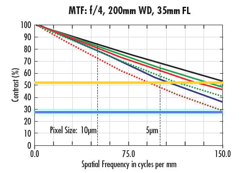
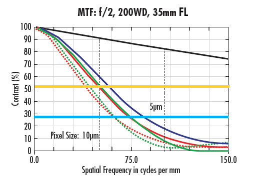
Figure 4: MTF curves for a 35mm lens at the same WD and different f/#s: f/4 (a) and f/2 (b).
Ex. 4: The Effect of Changing Working Distance on MTF
For Figure 5, WDs of 200mm (a) and 450mm (b) are examined for the same 35mm lens design at f/2. The large performance difference is directly related to the ability to balance aberrational content in a lens design over a range of WDs. Changing WD, even with refocusing, will lead to variations or reductions in performance as the lens moves away from its designed range. These effects are most profound at lower f/#s.
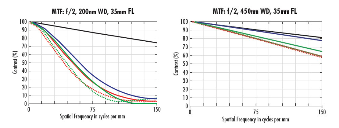
Figure 5: MTF curves for a 35mm focal length lens at f/2 with different WDs.
Wavelength Effects on Performance
Different wavelengths bend at different angles as light passes through a medium (glass, water, air, etc.). This is seen when sunlight passes through a prism and creates a rainbow effect; shorter wavelengths are bent more than longer ones. This same effect complicates resolution and information gathering in imaging systems. To avoid this issue, imaging and machine vision systems use monochromatic (single wavelengths) or narrow waveband illumination. Monochromatic illumination (e.g. from a 660nm LED) practically eliminates chromatic aberrations from an imaging system.
Chromatic Aberrations
Chromatic aberrations exist in two forms: lateral color shift (Figure 6) and chromatic focal shift (Figure 7).
Lateral color shift, Figure 6, is seen by moving from the center of an image towards the edge of the image. In the center, the spots for different wavelengths of light are concentric. Moving towards the corner of the image, wavelengths separate and produce a rainbow effect. Because of color separating, a given point on the object is imaged over a larger area, resulting in reduced contrast. On sensors with smaller pixels, this result is even more pronounced, as the blurring spreads over more pixels. Details on lateral color can be found in Aberrations on aberrations.

Figure 6: A depiction of a spot experiencing lateral color shift at different field points.
Chromatic focal shift, Figure 7, relates to the ability of a lens to focus all wavelengths at the same distance away from the lens. Different wavelengths will have different planes of best focus. This shift in focus with respect to wavelength results in reduced contrast since the different wavelengths create different spot sizes at the image plane where the camera sensor is located. In the image plane of Figure 7 a small spot size in the red wavelengths, a larger spot size in green, and the largest spot size in blue is shown. Not all colors will be in focus all at once. Advanced details can be found in Aberrations on aberrations.

Figure 7: A depiction of a spot experiencing chromatic focal shift at different depths.
Choosing the Optimal Wavelength
Monochromatic illumination enhances contrast by eliminating both chromatic focal shift and lateral chromatic aberration. Consider using LED illumination, lasers, or filters. However, different wavelengths can have different MTF effects in a system. The diffraction limit defines the smallest theoretical spot that can be created by a perfect lens, as defined by the Airy disk diameter, which has a wavelength (λ) dependence. Using Equation 1, one can analyze the change in spot size for both different wavelengths and different f/#s.
Table 1 features the calculated Airy disk diameter for wavelengths ranging from violet (405nm) to near-infrared (880nm) at various f/#s. This data shows that lens systems have better theoretical resolution and performance when used with shorter wavelengths. Shorter wavelengths allow for better use of the sensor’s pixels regardless of size due to the smaller achievable spot size. This is especially pronounced on sensors with very small pixels. Using higher f/#s allows for greater DOF. A red LED can be used at f/2.8 to generate a spot size of 4.51µm or a blue LED can generate almost the same spot size at f/4. If both options yield acceptable levels of performance at best focus, the system set at f/4 using blue light will produce better DOF, which could be a critical requirement.
| Color | Wavelength | Aperutre (f/#) | ||||
|---|---|---|---|---|---|---|
| f/1.4 | f/2.8 | f/4 | f/8 | f/16 | ||
| NIR | 880 | 3.01 | 6.01 | 8.59 | 17.18 | 34.36 |
| Red | 660 | 2.25 | 4.51 | 6.44 | 12.88 | 25.77 |
| Green | 520 | 1.78 | 3.55 | 5.08 | 10.15 | 20.30 |
| Blue | 470 | 1.61 | 3.21 | 4.59 | 9.17 | 18.35 |
| Violet | 405 | 1.38 | 2.77 | 3.95 | 7.91 | 15.81 |
Table 1: Theoretical Airy disk diameter spot sizes for various wavelengths and f/#s.
Ex. 5: Improvement with Wavelength
Both images in Figure 8 are taken with the same lenses and camera producing the same FOV, thus presenting the same spatial resolution on the object. The camera utilizes 3.45µm pixels. The illumination in Figure 8a is set at 660nm and 8b at 470nm. The high-resolution lens was set to a higher f/# to greatly reduce any aberrational effects. This allows diffraction to be the primary limitation in the system. The blue circles show the limiting resolution in Figure 8a. Note that Figure 8b has a significant increase in resolvable detail (approximately 50% finer detail). Even at the lower frequencies (wider lines), there is a higher level of contrast with 470nm illumination in Figure 8b.
Figure 8: Images of the star target taken with the same lens, at the same f/#, with the same sensor. The wavelength is varied from 660nm (a) to 470nm (b).
Ex. 6: White Light vs. Monochromatic MTF
In Figure 9, the same lens is used at the same WD and f/#. Figure 9a is showing white light, and Figure 9b is showing 470nm illumination. In Figure 9a, the performance is at 50% of the Nyquist limit (for a 3.45 μm pixel) or below. For Figure 9b, the performance at the Nyquist limit is higher than Figure 9a. Additionally, performance in the center of the system in Figure 9b is above the diffraction limit of Figure 9a. The reason for this increase in performance is twofold: using monochromatic light eliminates chromatic aberrations which allows for smaller spots to be created, and 470nm illumination is one of the shortest wavelengths of light used in the visible range for imaging. As detailed in the sections on diffraction limit and Airy disk, shorter wavelengths allow for higher resolution.
Figure 9: MTF curves for the same lens at f/2 using different wavelengths; white light (a) and 470nm (b).
Wavelength Considerations
A few issues can arise with changing wavelength. Lens designs can struggle the more the wavelength of the illumination trends in the UV direction (as wavelength decreases), regardless of if the waveband is narrow: glass materials tend not to perform as well at shorter (lower than about 425 nm) wavelengths. Designs do exist in this region of the spectrum, but they are often limited in capabilities, and the rare materials used require the lens build to be costlier. The best theoretical performance seen in Table 1 is at the violet wavelength of 405nm, but most system designs cannot perform well in this area. It’s very important to evaluate what a lens can realistically do at such short wavelengths using lens performance curves.
Ex. 7: Theoretical Limitations
Figure 10 compares a 35mm lens at f/2 with blue (470nm) and violet (405nm) wavelengths (10a and 10b respectively). While Figure 10a has a lower diffraction limit, it also shows that the 470nm wavelength yields higher performance at all field positions. The effect here is increased when the lens is used at the extremes of its design capabilities for f/# and WD (detailed in The Modulation Transfer Function on MTF). Another wavelength issue that can greatly affect performance is related to chromatic focal shift. As the application’s wavelength range increases, the lens’s ability to maintain high levels of performance will be compromised. Aberrations on aberrations goes into more detail on the phenomenon.


or view regional numbers
QUOTE TOOL
enter stock numbers to begin
Copyright 2023 | Edmund Optics, Ltd Unit 1, Opus Avenue, Nether Poppleton, York, YO26 6BL, UK
California Consumer Privacy Acts (CCPA): Do Not Sell or Share My Personal Information
California Transparency in Supply Chains Act
This content may include material that has been generated or modified using artificial intelligence (AI).
The FUTURE Depends On Optics®