


Comparison of Optical Aberrations
Identifying Aberrations | Aberration Examples
Optical aberrations are deviations from a perfect, mathematical model. It is important to note that they are not caused by any physical, optical, or mechanical flaws. Rather, they can be caused by the lens shape itself, or the placement of optical elements within a system, due to the wave nature of light. Optical systems are typically designed using first-order or paraxial optics in order to calculate image size and location. Paraxial optics does not take into account aberrations; it treats light as a ray and therefore omits the wave phenomena that cause aberrations. For an introduction on optical aberrations, view Chromatic and Monochromatic Optical Aberrations.
After defining the different groups and types of chromatic and monochromatic optical aberrations, the difficult part becomes recognizing them in a system, either through computer analysis or real-world observation, and then correcting the system to reduce the aberrations. Typically, optical designers first put a system into optical system design software, such as Zemax® or Code V®, to check the performance and aberrations of the system. It is important to note that after an optical component is made, aberrations can be recognized by observing the output of the system.
Optically Identifying Aberrations
Determining what aberrations are present in an optical system is not always an easy task, even when in the computer analysis stage, as commonly two or more aberrations are present in any given system. Optical designers use a variety of tools to recognize aberrations and try to correct them, often including computer-generated spot diagrams, wave fan diagrams, and ray fan diagrams. Spot diagrams illustrate how a single point of light would appear after being imaged through the system. Wave fan diagrams are plots of the wavefront relative to the flattened wavefront where a perfect wave would be flat along the x-direction. Ray fan diagrams are plots of points of the ray fan versus pupil coordinates. The following menu illustrates representative wave fan and ray fan diagrams for tangential (vertical, y-direction) and sagittal (horizontal, z-direction) planes where $ \small{H = 1} $ for each of the following aberrations: tilt $ \left( \small{W_{111}} \right) $, defocus $ \left( \small{W_{020}} \right) $, spherical $ \left( \small{W_{040}} \right) $, coma $ \left( \small{W_{131}} \right) $, astigmatism $ \left( \small{W_{222}} \right) $, field curvature $ \left( \small{W_{220}} \right) $, and distortion $ \left( \small{W_{311}} \right) $. Simply select the aberration of interest to see each illustration.
Aberration Name (Wavefront Coefficient):
Figure 1: Airy Disk Pattern
Recognizing aberrations, especially in the design stage, is the first step in correcting for them. Why does an optical designer want to correct for aberrations? The answer is to create a system that is diffraction-limited, which is the best possible performance. The aberrations of diffraction-limited systems are contained within the Airy disk spot size, or the size of the diffraction pattern caused by a circular aperture (Figure 1).
Equation 1 can be used to calculate the Airy disk spot size $ \small{\left( d \right)} $ where $ \small{\lambda} $ is the wavelength used in the system and f/# is the f-number of the system.
OPTICAL ABERRATION EXAMPLES
After a system is designed and manufactured, aberrations can be observed by imaging a point source, such as a laser, through the system to see how the single point appears on the image plane. Multiple aberrations can be present, but in general, the more similar the image looks to a spot, the fewer the aberrations; this is regardless of size, as the spot could be magnified by the system. The following seven examples illustrate the ray behavior if the corresponding aberration was the only one in the system, simulations of aberrated images using common test targets (Figures 2 - 4), and possible corrective actions to minimize the aberration.
Simulations were created in Code V® and are exaggerated to better illustrate the induced aberration. It is important to note that the only aberrations discussed are first and third orders, due to their commonality, as correction of higher-order aberrations becomes very complex for the slight improvement in image quality.
Figure 2: Fixed Frequency Grid Distortion Target
Figure 3: Negative Contrast 1951 USAF Resolution Target
Figure 4: Star Target
| Tilt – $\small{W_{111}}$ |
|
 Figure 5a: Representation of Tilt Aberration |
 Figure 5b: Simulation of Tilt Aberration |
Characterization
|
Corrective Action
|
| Defocus – $\small{W_{020}}$ | |
 Figure 6a: Representation of Defocus Aberration |
 Figure 6b: Simulation of Defocus Aberration |
Characterization
|
Corrective Action
|
| Spherical – $\small{W_{040}}$ | |
 Figure 7a: Representation of Spherical Aberration |
 Figure 7b: Simulation of Spherical Aberration |
Characterization
|
Corrective Action
|
| Coma – $\small{W_{131}}$ | |
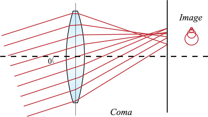 Figure 8a: Representation of Coma Aberration |
 Figure 8b: Simulation of Coma Aberration |
Characterization
|
Corrective Action
|
| Astigmatism – $\small{W_{222}}$ | |
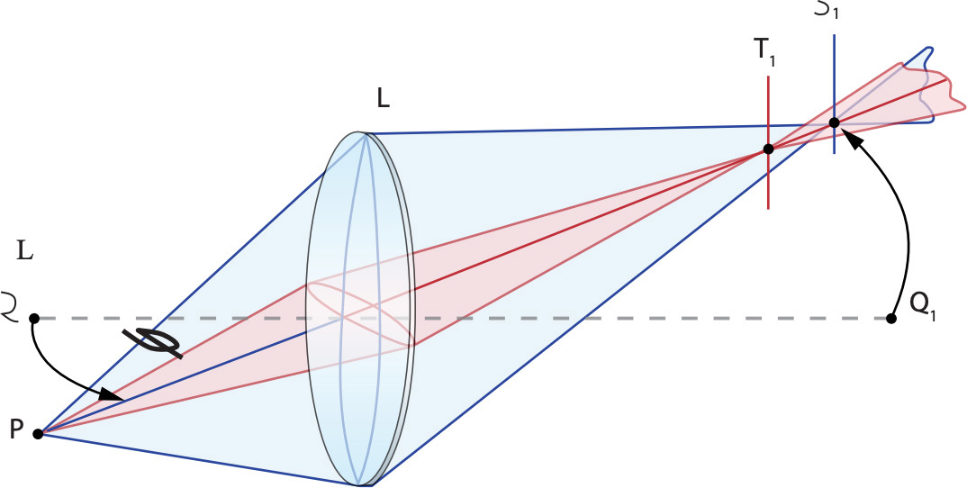 Figure 9a: Representation of Astigmatism Aberration |
 Figure 9b: Simulation of Astigmatism Aberration |
Characterization
|
Corrective Action
|
| Field Curvature – $\small{W_{220}}$ | |
 Figure 10a: Representation of Field Curvature Aberration |
 Figure 10b: Simulation of Field Curvature Aberrationn |
Characterization
|
Corrective Action
|
| Distortion – $\small{W_{311}}$ | |
 Figure 11a: Representation of Distortion Aberration |
Figure 11b: Simulation of Barrel Distortion Aberration 
Figure 11c: Simulation of Pincushion Distortion Aberration |
Characterization
|
Corrective Action
|
Recognizing optical aberrations is very important in correcting for them in an optical system, as the goal is to get the system to be diffraction limited. Optical and imaging systems can contain multiple combinations of aberrations, which can be classified as either chromatic or monochromatic. Correcting aberrations is best done in the design stage, where steps such as moving the aperture stop or changing the type of optical lens can drastically reduce the number and severity (or magnitude) of aberrations. Overall, optical designers work to reduce first and third-order aberrations primarily because reducing higher-order aberrations adds significant complexity with only a slight improvement in image quality.
Reference
- Dereniak, Eustace L., and Teresa D. Dereniak. Geometrical and Trigonometric Optics. Cambridge: Cambridge University Press, 2008.


or view regional numbers
QUOTE TOOL
enter stock numbers to begin
Copyright 2023 | Edmund Optics, Ltd Unit 1, Opus Avenue, Nether Poppleton, York, YO26 6BL, UK
California Consumer Privacy Acts (CCPA): Do Not Sell or Share My Personal Information
California Transparency in Supply Chains Act
This content may include material that has been generated or modified using artificial intelligence (AI).
The FUTURE Depends On Optics®