Propagation of a Gaussian Beam Through a Thin Lens

Understanding Gaussian beam propagation is fundamental to optical design in many laser-based applications. Many laser beams exhibit a Gaussian intensity profile because the transverse modes of optical resonators are described by Hermite-Gaussian or Laguerre-Gaussian functions, with the fundamental (lowest-order) mode corresponding to a pure Gaussian distribution.

This application note introduces the key properties of Gaussian beams and examines how propagation through a thin lens affects key beam parameters, including beam size, divergence, and waist position. The following sections follow the standard textbook treatment commonly found in the references listed below.

Gaussian Beam: Definition and Characteristics

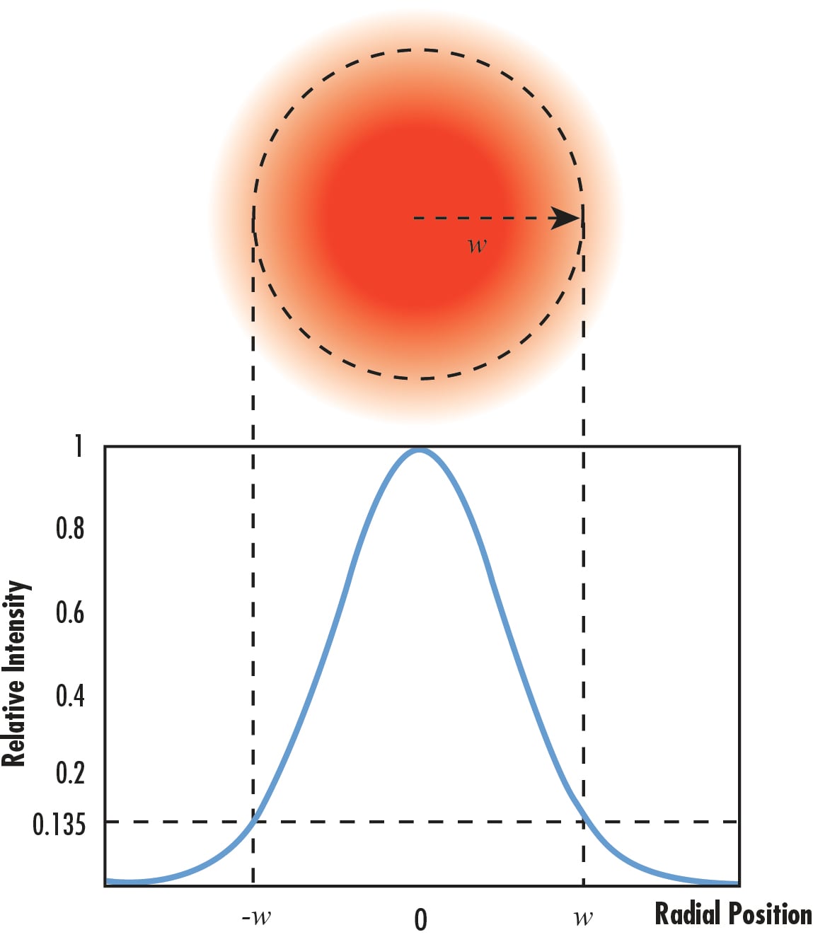
Gaussian irradiance profiles are symmetric around the beam axis and decrease with increasing radial distance from the center (Figure 1). The transverse optical intensity as a function of radial distance 𝑟 is expressed as:

where \({I}_{0}\) is the peak irradiance at the beam axis, \(P\) is the total power of the beam and \(w\) is the beam radius at which the irradiance falls to \(1/{e}^{2}\) (~13.5%) of \({I}_{0}\).

Beam Caustic in Gaussian Beam Propagation

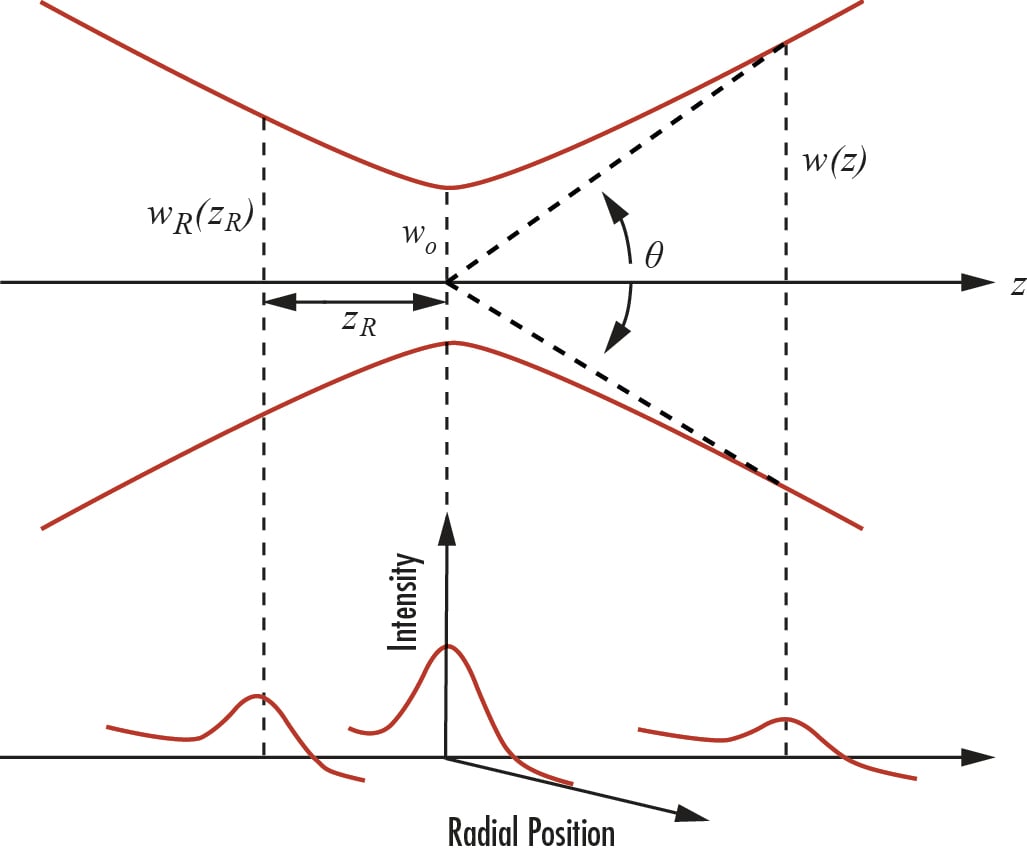
The irradiance profile of a Gaussian beam changes as it propagates through space. Due to diffraction, the beam converges and diverges around the beam waist where the beam diameter reaches its minimum value \(2{w}_{0}\). The path of the beam diameter from and to its waist is also known as the beam caustic (Figure 2).

The beam radius as a function of propagation distance \(z\) is given by the following equation:

Here \({z}_{R} \) denotes the Rayleigh length, a characteristic distance of the beam. At the beam waist location (\(z=0\)), the intensity reaches its absolute maximum \(\frac{2P}{π{w}_{0}^{2}}\) on the beam axis. The Rayleigh length represents the distance from the waist at which the beam radius increases by a factor of \(\sqrt{2}\) corresponding to a reduction of the peak intensity by a factor of two.

Rayleigh Length and Divergence in Gaussian Beams

In the far field limit (\(z≫{z}_{R}\)), the beam radius increases linearly with \(z\), allowing the divergence angle \(θ\) to be defined as:

Rayleigh length and divergence angle are all quantities that are intrinsically linked to one another. Combining Equations 3 and 4 yields:

where \(λ\) is the wavelength of the beam. Equation 5 shows that a smaller beam waist leads to a larger divergence angle, and vice versa.

Beam Quality Metrics for Gaussian Beams

The product \({w}_{0}θ\) is known as the beam parameter product (\(BPP\)). It is an inherent property of the beam and a measure of beam quality. Another measure of beam quality is the M²factor that can be defined as the ratio of the beam parameter products of the real beam to that of a diffraction-limited Gaussian beam with the same wavelength.

This has a significant implication on optical design as an optical system can be optimized either for beam waist size or for beam divergence, but not independently for both. For example, it is impossible to generate an arbitrarily small collimated beam. Another practical case is coupling a beam into a fiber: depending on the fiber NA and core diameter, poor beam quality can compromise the coupling efficiency into the fiber.

Beam quality may also be interpreted as a measure of how closely the beam wavefronts resemble those of an ideal diffraction-limited Gaussian beam. We will now examine how the curvature of Gaussian beam wavefronts evolves during propagation.

Radius of Curvature of Gaussian Wavefronts

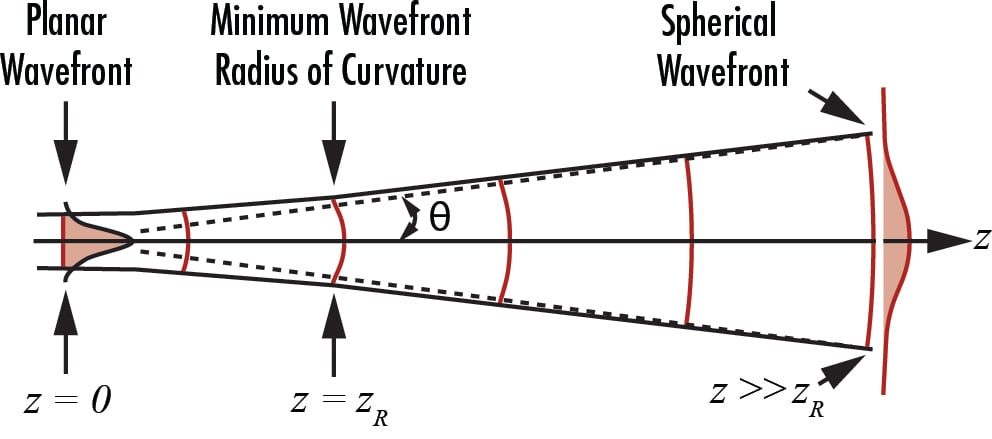
At the beam waist the radius of curvature is \(R→∞\), corresponding to a planar wavefront. As the beam propagates away from the waist, the curvature increases, reaching a minimum value of \(R=2{z}_{R}\) at \({z}_{R}\). For \(z≫{z}_{R}\), \(R\) increases linearly with \(z\) and the wavefront becomes nearly spherical (Figure 3).

Describing the Propagation of a Gaussian Beam

To describe a Gaussian beam completely, it’s enough to know two independent parameters of the beam, for example, the waist position and size, or alternatively, the beam radius and wavefront curvature at a certain point. Let’s show the latter explicitly, since it will be useful in the next section.

By combining Equations 2, 3 and 6 we can determine the axial position \(z\) from the beam waist where the beam has a wavefront curvature \(R\) and beam radius \(w\):

The Complex q Parameter

Knowing the waist position and size (or equivalently the Rayleigh length) is sufficient to fully describe the spatial evolution of a Gaussian beam. With that in mind it is useful to introduce the complex q parameter of the beam:

The complex q parameter contains all the information about the beam, and it can be used in combination with ABCD matrices to propagate the beam through any aberration-free optical system.

The ABCD matrices used with Gaussian beams are the same as in ray optics. For a thin lens the ABCD matrix has the following form:

Equation 13 is known as the Gaussian thin lens equation. In the following paragraph, we derive the same equation using a slightly different approach to emphasize its correspondence with the thin lens equation in ray optics.

Gaussian Beam Propagation Through a Thin Lens

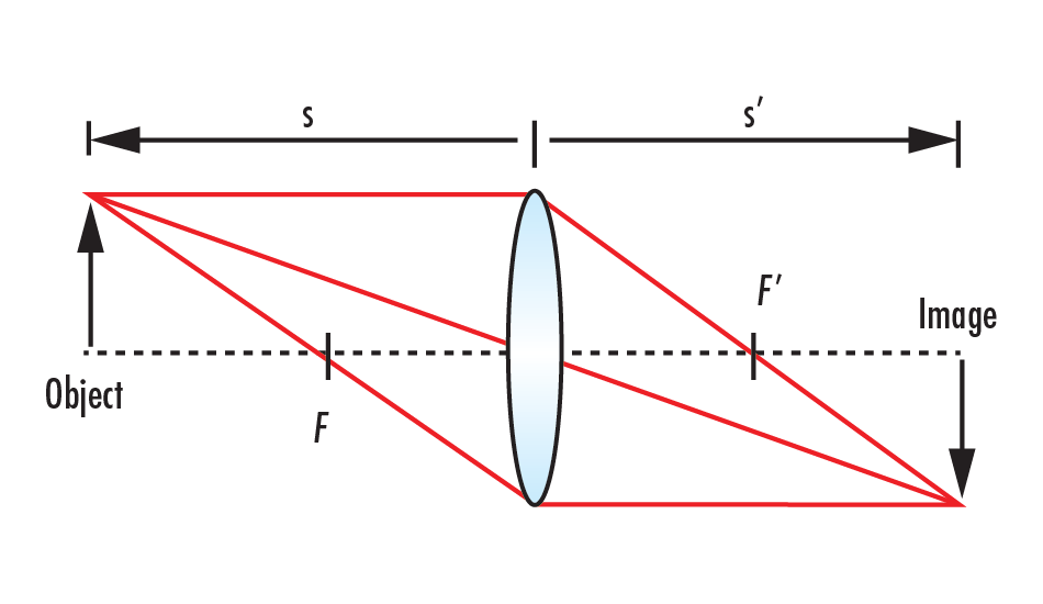
Many laser applications require manipulation of a laser beam as opposed to simply using the “raw” beam. This may be done using optical components such as lenses, mirrors, prisms, and more. In this section, we examine how a thin lens modifies the Gaussian beam parameters. Let’s first recall the lens equation which describes the behavior of a thin lens in geometric optics:

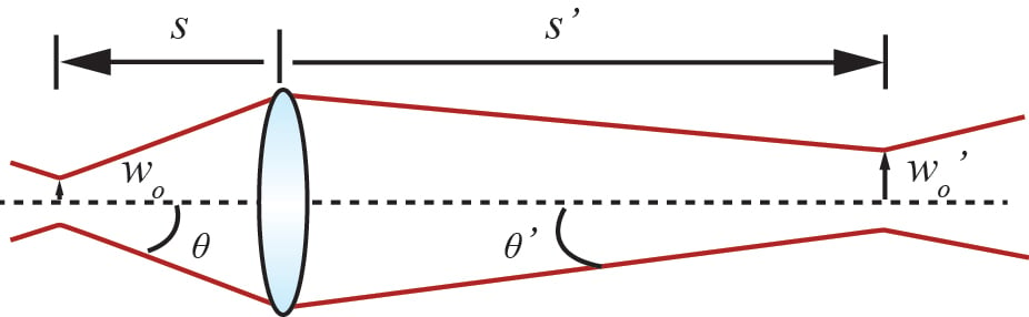
In Equation 14, \(s\) is the object distance, \(s\)’ is the image distance, and \(f\) is the focal length of the lens (also see Figure 4). The intrinsic signs of 𝑠 and 𝑠’ depend on whether the object or image lies in the object or image half-plane: they are positive if the object (image) lies in its respective half-plane and negative otherwise.

For reasons that will become clear in the next paragraph it is useful to express Equation 14 in a dimensionless form by multiplying both sides by \(f\):

Now, let’s consider a Gaussian beam incident on a thin lens, as illustrated in Figure 5. Because the lens thickness is negligible, the beam radius immediately before and after the lens can be assumed to be unchanged (\(w=w’\)). The curvature of the lens introduces however an additional phase shift, and the wavefront curvature of the transmitted beam \(R’\) is related to the incident curvature \(R\) by:

As shown by Equations 7 and 8, knowing the beam radius and curvature at a given location completely determines the beam. This allows us to derive the location of the output waist \(s'\) as a function of the input waist position \(s\) with respect to the lens:

Equation 17 becomes identical to Equation 13 by introducing the following coordinate transformation: s becomes z, s’ becomes -z’. In this new coordinate system, the reference frame of each beam is defined relative to its respective beam waist. When \(\left( s-f \right)≫{z}_{R}\), meaning when the waist position is far from the focal point of the lens in Rayleigh length units, Equation 15 is recovered.

Effect of Rayleigh Length on the Imaged Waist

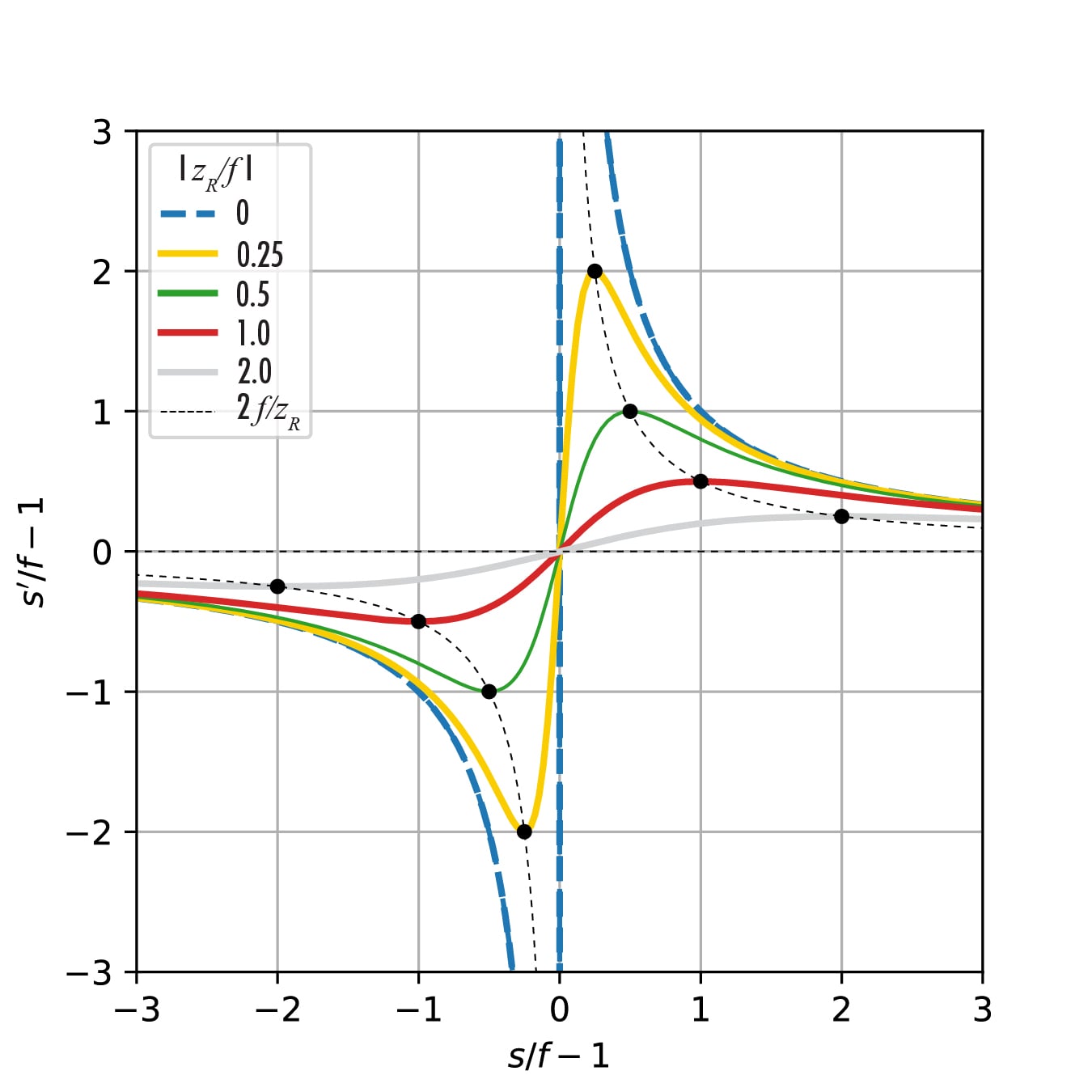
A plot of the normalized image distance versus the normalized object distance shows the effect of the Rayleigh range on the location of the imaged waist (Figure 6). Unlike ray optics, where the image moves to infinity when \(s=f,\) in Gaussian optics the waist moves to \(f\). The maximum distance of the imaged waist from the lens is given by

When the Rayleigh length is small, the waist location of the imaged beam moves toward infinity. Conversely, when the Rayleigh length is large, the waist location approaches the focal length \(f\).

Transformation of Gaussian Beams after a Thin Lens

To fully understand how Gaussian beams transform after passing through the lens, we also need to know how the beam waist or alternatively the Rayleigh range changes.

Following the same approach used to obtain Equation 17, it is possible to derive a relation between the input and output waist sizes:

In Equation 20 we have introduced another important parameter of the optical system which is the magnification factor \(α\) of the lens.

In some cases, it is convenient to rewrite Equation 17 in terms of the magnification factor:

Since the beam parameter product \(BPP={w}_{0}θ\) is conserved, the beam divergence transforms as:

The magnification factor is therefore the key parameter governing the beam transformation during propagation through the lens.

If \(|s-f|≪{z}_{R}\) the magnification tends to \(\left| f/{z}_{R} \right|\). As expected for \(\left| s-f \right|≫{z}_{R}\) we simply recover the magnification factor of the lens known in geometrical optics \({α}_{R}=\left| \frac{f}{s-f} \right|\). Note that geometrical optics represents the upper limit of the lens magnification (\(α<{α}_{R}\)).

Gaussian Beam Focusing and Collimation

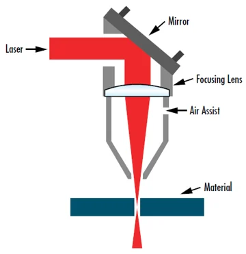
In many applications, such as laser materials processing or surgery, it is highly important to focus a laser beam down to the smallest spot possible to maximize intensity and minimize the heated area (Figure 7).

In other cases, the goal is reversed, for example when a diverging beam (such as the beam from a single-mode fiber) should be collimated. The equations introduced in the previous section are particularly useful for both cases. Consider a lens placed at the waist of a Gaussian beam (\(s=0\)). In this configuration, Equations 17 and 20 become respectively:

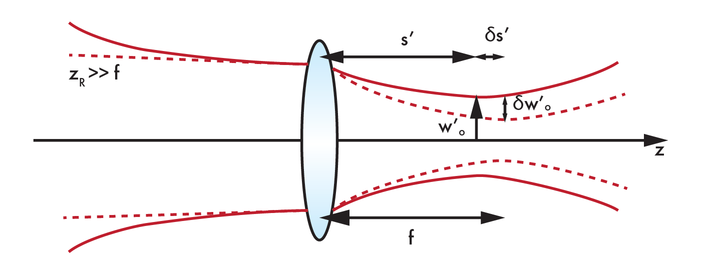
Although the wavefront is planar at the beam waist, a Gaussian beam with a waist at the lens position does not behave exactly like a plane wave. As illustrated in Figure 8, the new waist (\({w'}_{0}\)) does not coincide precisely with the geometrical focus predicted by ray optics. This deviation originates from the finite divergence of the Gaussian beam, or equivalently, from its finite transverse intensity distribution, which causes the beam waist to form slightly away from the geometric focal plane.

In geometrical optics, by contrast, the divergence (\(\frac{λ}{π{w}_{0}}\)) can be zero. In the limit (\(λ≪ {w}_{0}\)), we retrieve the results predicted by geometrical optics. Since laser wavelengths are typically much smaller than the beam waist, the ray-optics approximation is often sufficiently accurate for many practical applications.

Now consider a collimated beam to be focused on a workpiece. A beam is collimated if the beam radius doesn’t change within a certain propagation distance. This condition is fulfilled when the Rayleigh range is much larger than the focal length: \({z}_{R}≫f\).

The magnification factor is just \(|f/{z}_{R}|\), and the output waist is located at the focal plane of the lens (\({s}^{'}=f\)). Equations 24 and 26 simplify to

respectively. These results are consistent with those obtained for a set of parallel rays incident on the lens: the focused spot is determined solely by the focal length and the input beam diameter. In this geometric limit, the exact waist location of the input beam is irrelevant because the beam’s radius and wavefront curvature are nearly constant, and the concept of waist loses its significance.

Equation 27 shows that the spot size can be minimized by reducing the lens’ focal length and by decreasing the beam divergence (or equivalently, increasing the beam radius). To make sure the lens can capture the full beam energy, the diameter \(D\) of the lens is usually set to be four times the beam radius and therefore the numerical aperture of the lens is \(NA=\frac{D}{f}=4{w}_{0}/f\). Equation 27 can be written in terms of NA as:

This expression shows that the focused spot diameter is inversely proportional to the numerical aperture of the focusing system.

Due to the reversibility of optical systems, the results derived for focusing a collimated beam can be directly applied to the collimation of a diverging beam. It is sufficient to exchange the object and image half-spaces.

A commonly misunderstood point is that achieving a collimated beam does not require driving \(s'\) to infinity. Rather, the condition for optimal collimation is to minimize the Rayleigh range \({z'}_{R}\), which is equivalent to minimizing the output beam divergence (\(θ'\)). As shown in the previous section, when \(s=f\), the image distance \(s'\) approaches \(f\), not infinity. Therefore, long focal-length lenses combined with highly diverging input beams (i.e., large (\(|f/{z}_{R}|\))) produce better collimation and lower output divergence. However, because the beam parameter product is conserved, improved collimation comes at the expense of a larger output beam diameter.

Summary and Key Takeaways

This application note highlights the characteristics of a Gaussian laser beam and its propagation through a thin lens. The analysis in the text also explains how Gaussian beam propagation departs from simple geometric optics and why a wave-based description is essential for accurately predicting beam behavior. The resulting relations clarify how waist size, waist position, and divergence evolve after a lens, providing a rigorous basis for optimizing both focusing and collimation. This knowledge is crucial whenever precise control over beam quality or spot size is required, ensuring that optical system design aligns with the fundamental constraints of Gaussian beam physics. More information on laser beam quality or beam parameters can be found in the application note Beam Quality and Strehl Ratio. For an overview of laser beam shaping products please refer to our Beam Shapers product page.

References

Saleh, B. E. A., & Teich, M. C. (2019). Fundamentals of photonics (3rd ed., Vol. 1). Wiley.
Siegman, A. E. (1986). Lasers. University Science Books.
Self, Sidney A. “Focusing of Spherical Gaussian Beams.” Applied Optics, vol. 22, no. 5, January 1983.
Please select your shipping country to view the most accurate inventory information, and to determine the correct Edmund Optics sales office for your order.
Previous Section
or view regional numbers
QUOTE TOOL
enter stock numbers to begin
Copyright 2023 | Edmund Optics, Ltd Unit 1, Opus Avenue, Nether Poppleton, York, YO26 6BL, UK
California Consumer Privacy Acts (CCPA): Do Not Sell or Share My Personal Information
California Transparency in Supply Chains Act
This content may include material that has been generated or modified using artificial intelligence (AI).
The FUTURE Depends On Optics®